


Intro
There are as many strategies for extracting alpha from the markets as there are traders. Unfortunately, this article will be discussing none of them. If that’s what you’re looking for, I suggest you check out the very sophisticated techniques covered in this video.
OK. If you’re still reading, you probably take trading at least somewhat seriously. When setting up your trading business (and it is a business, like any other), one of the most important things to consider is the impact that costs will have on your bottom line. And just like any other business, traders deal with costs in many forms. This article will discuss the explicit and implicit costs that are incurred on every transaction in global markets. We’ll apply this primer to a real world application for the cryptocurrency derivatives exchange Bitmex, with its unique properties. Finally, we’ll develop a simple execution algorithm that should help to reduce the impact costs have on our PnL. If any of that sounds remotely interesting or useful, read on!
Notebook for this article can be found here.
Explicit (Fixed) Costs
Fixed costs, comprised mainly of commissions and fees, are quoted in advance by the exchange or broker where orders are placed. These fees serve as compensation for the service of matching buyers with sellers. These costs differ depending on which venue traders use to execute their trades, and typically come in one of the following forms:
-
- Constant cost per share/contract
- Constant cost per trade
- Cost as a percentage of total trade value
These fees can sometimes be negotiated with one’s broker, and there are often discounts/tiered pricing for traders who do more volume. However, the influence a trader has on these fees is mostly limited. That said, commissions have come down dramatically in recent years, and brokerages such as Robinhood and Alpaca even offer commission-free trading.
Implicit (Variable) Costs
Depending on the volume a trader executes relative to the overall market, implicit variable costs can be a much more significant part of their bottom line. These consist primarily of market impact, timing risk and price trend, but also include spreads and opportunity costs. Market impact and spread costs affect those executing aggressively (taking liquidity), while passive traders (liquidity providers) are more concerned with timing risk and price trend.
The most obvious variable cost is the Bid/Ask spread. Wider spreads offer less favorable prices for those requiring liquidity to enter/exit the market. In most liquid markets under normal conditions, spreads are typically one tick wide. However, these spreads can widen dramatically during periods of high volatility or illiquidity. Also worth noting is that in instruments such as spot FX and CFDs the broker themselves, rather than other market participants, are the counterparties to all trades. In these cases, spreads are determined directly by the brokerage, not liquidity providers/market makers.
Market impact represents the change in market price caused by the execution of an order and has both temporary and permanent components. This cost is determined by the quantity desired from the trader taking liquidity, and the liquidity available in the market. A trader wishing to buy a single share of Apple stock is affected significantly less than one attempting to purchase 1 million barrels’ worth of crude oil futures contracts. The temporary market impact is the immediate result of liquidity being removed from the market. For example, if there are 100 contracts on each of the first 10 levels of the Limit Order Book and a trader places a market order for 700 contracts, the price will immediately jump 7 ticks. However, as this is likely an unusually large order, we would expect price to revert somewhat after it’s filled. The permanent impact is a function of where price settles after the order clears. A plausible scenario is that 30 seconds later, the market has retraced to within 2 ticks of where it started. This reflects the fact that a trader placing such a large, urgent order probably has information that other participants aren’t yet privy to, and the price has adjusted to discount this. Temporary market impact is typically reduced by splitting large orders into smaller slices (although apparently no one on Bitmex got the memo, where traders are wont to take out 20+ levels of resting liquidity with a single market order). Permanent market impact may be mitigated somewhat by slicing orders, but pronounced buying/selling activity will still likely affect price.
To avoid the costs described above, traders may opt for a more passive style. This typically includes the use of limit orders on the “near” side of the order book to reduce the impact their trading has on the market price. The costs and risk borne by these traders relate to the fact that their orders aren’t guaranteed to be filled. Whereas an aggressive trader will use all available liquidity to achieve their desired position, a passive trader is at the mercy of the market coming to them. The two main sources of uncertainty, therefore, are price volatility in both the asset’s price and its volume/liquidity (spreads may also be considered but are correlated to the two previous factors).
In this scenario, costs are occurred when price trends away from a resting limit order. This leaves the order unfilled. The trader must make the decision to either accept to accept the new (worse) price or wait to see if the market will revert. Choosing to execute in this passive manner also exposes the trader to the risk of changing volume/liquidity conditions. If they’re forced to become more aggressive in response to an adversely trending market, reduced liquidity at the time of execution can lead to greater market impact than would be experienced if they’d executed immediately. “A bird in the hand is worth two bushes”, as the saying goes (right?).
The optimal execution strategy then becomes a balancing act between these various costs. Should the trader take liquidity immediately, risking an adverse impact on market price? Or passively attempt to achieve a better price at the risk of not getting filled? There is also the discussion around adverse selection, whereby a trader who uses limit orders on the near side of the book will get filled on all their losing trades, but not all their winning ones; we won’t get into this here.
Bitmex-Specific Idiosyncracies
This primer brings us to the real-world example of Bitmex (the Bitcoin Mercantile Exchange), the world’s most liquid exchange for cryptocurrency derivatives, as per sk3w.co. Bitmex employs a maker-taker fee structure, whereby liquidity providers (“makers”) and liquidity “takers” are charged different fees to execute their orders. The table below shows the fee structure for all actively traded futures/swaps contracts listed on the exchange.
| Symbol | Maker Fee | Taker Fee |
| XBTUSD | -0.025% | 0.075% |
| XBTU19 | -0.025% | 0.075% |
| ETHUSD | -0.025% | 0.075% |
| ADAU19 | -0.05% | 0.25% |
| BCHU19 | -0.05% | 0.25% |
| EOSU19 | -0.05% | 0.25% |
| ETHU19 | -0.05% | 0.25% |
| LTCU19 | -0.05% | 0.25% |
| TRXU19 | -0.05% | 0.25% |
| XRPU19 | -0.05% | 0.25% |
Note that maker fees are actually negative; this indicates a rebate paid to compensate them for providing liquidity to the exchange. Note also that the fees on the first 3 products are lower than the remainder. This is because those products trade significantly more volume, thus requiring less incentive for market participants to provide liquidity. More revenue is also generated on an absolute basis, allowing them to cut traders some slack.
Another important exchange feature to highlight is that the minimum amount price is allowed to change by (the tick size) differs from contract to contract. This becomes relevant when considered as a percentage of the value of the contract itself. Larger tick sizes relative to price cause each individual change in price to be larger on a percentage basis. These values are summarized below (prices used are daily closes from August 15, 2019).
| Symbol | Price | Tick Size | Ratio |
| XBTUSD | 102855 | 0.5 | 0.00049% |
| XBTU19 | 10333.5 | 0.5 | 0.0048% |
| ETHUSD | 187.95 | 0.05 | 0.026% |
| ADAU19 | 0.00000457 | 0.00000001 | 0.22% |
| BCHU19 | 0.03037 | 0.00001 | 0.033% |
| EOSU19 | 0.0003491 | 0.0000001 | 0.029% |
| ETHU19 | 0.01814 | 0.00001 | 0.055% |
| LTCU19 | 0.007352 | 0.000005 | 0.068% |
| TRXU19 | 0.00000167 | 0.00000001 | 0.60% |
| XRPU19 | 0.00002537 | 0.00000001 | 0.039% |
Passive vs Aggressive Break-Evens
As discussed above, achieving optimal execution requires a balance between passive and active trading costs. For our purposes, we’ll consider a toy example where a trader has two options: market buy at the current best offer or place a limit order at the current best bid, continually adjusting as price moves up. We’ll consider the benchmark price to be the initial best offer. Assume that the bid/ask is always one tick wide and that price changes always occur in one tick increments. The costs in these two scenarios are as follows:
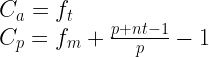
where:
Ca = the cost associated with aggressive execution
Cp = the cost associated with passive execution
ft = taker fee
fm = maker fee
p = benchmark price
n = number of ticks price best offer has moved from benchmark price
t = tick size
*these equations change slightly for inverse contracts such as XBTUSD, as well as for short positions. The differences to results aren’t significant. Functions for both are included in notebook
Given that maker fees are always less expensive and we’re placing our order on the near side of the LOB, this will result in the most favorable execution *if we are filled*. However, if price moves away from our order before we’re filled, executing at this less favorable price could prove to be more costly. With these equations defined, we can examine the break-evens; the price at which passive execution incurs greater overall costs than aggressive. Tick size plays a significant role in this calculation, so we’ll consider the two contracts with the most extreme tick/price ratios: namely XBTUSD and TRXU19.


These charts illustrate the impact of differences in both tick/price ratio and fee structure between the two contracts. The price of XBTUSD must move much farther (in tick terms) for passive execution to become more expensive than aggressive. This has direct implications for traders in these products. By solving for where these two lines intersect, we arrive at the number of ticks where passive execution becomes more expensive. This is calculated with the following equation:

We can use this to calculate the break-evens for all of the contracts offered on the exchange:
| Symbol | Break-Even (Ticks) |
| XBTUSD | 21.6 |
| XBTU19 | 21.7 |
| ETHUSD | 4.8 |
| ADAU19 | 2.4 |
| BCHU19 | 10.1 |
| EOSU19 | 11.5 |
| ETHU19 | 6.4 |
| LTCU19 | 5.4 |
| TRXU19 | 1.5 |
| XRPU19 | 8.6 |
Estimating Timing Risk
We now know how far price can run away from us before trying to achieve a better fill price and reducing fees bites us in the ass. However, we still need to know how likely it is that these break-evens will be breached before we get filled. This question has no closed solution; that would require perfect information about the future. To solve this problem, we’ll turn to simulation to attempt to determine a range of possible outcomes.
I’ll preface this simulation with a disclaimer. I’m going to make some assumptions that likely don’t completely describe true market behavior, but I think provide a useful framework for exploring this problem in a way that’s robust and easy to understand.
Let’s consider a random-walk process, where the next change in market price is either one tick up or one tick down. This change in last-traded price will correspond to either 1) a jump from best bid to best ask (or vice versa) or 2) the bid/ask both shifting by one tick as all liquidity at that price is taken. For our simple passive execution algorithm, we’ll stay on the best bid until we get filled or it moves away from us. To be guaranteed a fill using this model, we need two consecutive price changes towards our limit order (in the case of a buy order, two decreases).
To estimate how far we should expect price to run, we’ll perform a Monte Carlo analysis. This will generate thousands of potential random walks, paths that price could take after we place our order. We let each of these paths play out until we experience two consecutive ticks in our favor, ensuring our order would’ve been filled. After running this simulation many times and recording the final excursion from our target price (where we’d get filled), we end up with a distribution of outcomes. This distribution allows us to estimate the probability of getting filled before price moved n ticks away. It’s well-documented that the market is not a perfect random walk. To compensate for this, we can introduce auto-correlation into the process; that is, the probability that the next tick will be up given that the previous one was up and vice versa.
The following chart shows the results of running this simulation 50,000 times each, while varying the probability of consecutive ticks from 35% to 65%.

Optimal Execution Strategy/Algorithm
From the results of this simulation, if consecutive ticks are highly correlated (which makes intuitive sense when you consider situations where single market orders can clear multiple levels in the order book instantaneously), we would estimate that price will run away from us 5 ticks or less about 90% of the time. We can use this information to construct a basic execution algorithm for each contract.
Subtract 5 from each of the break-evens calculated previously. The result of this calculation is the price where we transition from passive to aggressive. Our algorithm will place a limit order at the top of the book, re-adjusting every time the bid/ask shifts. If price reaches the adjusted break-even, the attempt to get filled on the limit is abandoned, and a market order is placed. If the break-even is less than 5 ticks (ADA, TRX, and ETHUSD), this means that the optimal strategy is to place a market order immediately. If the assumptions of the simulations are reasonable, this basic strategy should strike a decent balance between fixed and variable trading costs, and improve our PnL (which is nice).
Conclusion/Future Work
Costs are something every trader must deal with. They’re also one of the few factors that are mostly within a trader’s control. Yet, they’re not as sexy as price action or indicators so little is focus is placed on them. With a better understanding of how costs are generated, we were able to develop a basic execution strategy that balances passive and aggressive costs.
However, this solution is by no means state-of-the art. As someone who isn’t responsible for executing tens of millions of dollars’ worth of orders, this basic solution suits me fine. For those whose job it is to get the very best execution possible, there is plenty more work to be done. Ideally, one would use L2/L3 data to analyze real changes in the order book, as well as market order flow. This would give a better sense of runs of consecutive ticks in one direction. Book pressure or imbalance also likely plays a significant role in which way a market is likely to break in the very near-term. Finally, considerations must be made for liquidity/volatility conditions in the market. During volatile periods, perhaps it’s best to execute aggressively for fear of the market rapidly trending away from a resting limit order. Or maybe there are times of the day where liquidity dries up and it’s worth a shot providing some. There are countless factors to consider, and market microstructure/execution is a study completely onto itself.
If you enjoyed this article (or didn’t), feel free to leave a comment below. You can also follow on Twitter @quantfiction, and/or join the Quant Talk Discord chat.